-The second algorithm uses intensity directional measurements and the parameters retrieved with the first “polarization algorithm” (i.e. scattering aerosol optical thickness and particles size). This method is described in details in Peers et al., (2015) : https://acp.copernicus.org/articles/15/4179/2015/acp-15-4179-2015.pdf.
The 7 aerosol models previously described for the “polarization algorithm” are still considered in this second algorithm. However, the imaginary part of the complex refractive (i.e. the aerosol absorption) is now included in the retrieval process as well as the cloud optical thickness. A LUT was also generated to compute the direct aerosol above cloud radiative forcing. Re-analysis data are also used to provide the wind speed, column integrated water amount and ozone.
The sources of errors for the AERO-AC products have been looked carefully in Peers et al., (2015). The figure 2 shows the errors in the AERO-AC retrieved parameters.
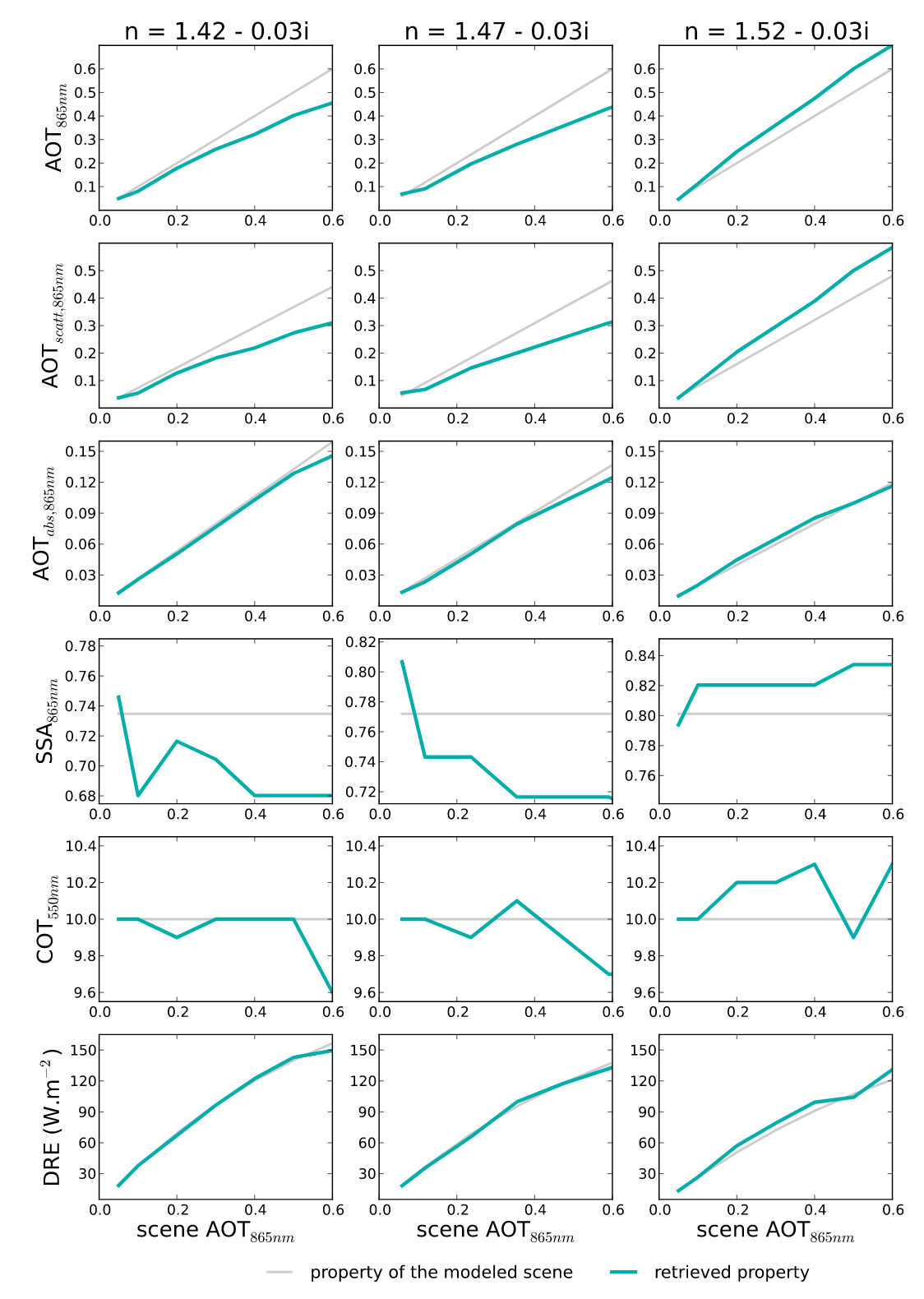
Figure 2 : Sensitivity of the properties of ACA conditions with different aerosol models. From top to the bottom: total AOT, scattering AOT, absorption AOT and SSA at 865 nm, COT at 550 nm and the shortwave DRE of aerosols. Grey lines correspond to the properties of the actual modeled conditions and green lines to those retrieved by the algorithm. The aerosol model of the first column has a refractive index n equal to 1.42−0.03i, the second, n=1.47−0.03i and the third, n=1.52−0.03i (source : Peers et al., 2015).